Deep Reinforcement Learning for Continuous Control

Let’s train an agent to control a robotic arm to continously track a moving target in the Reacher environment from Unity. We’ll combine deep neural networks and reinforcement learning using a multi-step variant of twin delayed deep determinsitic policy gradients (TD3 / DDPG) to teach an agent continous control. We’ll build up some theory for our methods and implement them to train and test an agent. Let’s dive in!

Figure 1: GIF animation showing agent trained to continously track a moving target using deep reinforcement learning (multi-step twin delayed deep determinstic policy gradients).

Here’s a full video showing the trained agent: https://youtu.be/JC9iwMmjpzo.

Outline

• The Environment
• Methods
  • Reinforcement Learning
  • Value-based Methods
  • Policy Gradients
  • Actor-Critic
  • Deep Deterministic Policy Gradients (DDPG)
    • Deterministic Policy Gradients
    • Experience Replay Buffer
    • Target Networks
    • Soft Updates
    • Batch Normalization
    • Exploratory Action Space Noise
  • Twin Deplayed DDPG (TD3)
    • Clipped Double Q-learning
    • Delayed Policy Updates
    • Target Policy Smoothing
  • Multi-Step Returns
• Implementation Details
• Training the Agent
• Testing the Agent
• Discussion & Next Steps

The Environment

The Reacher environment in Unity ML-Agents [1] features a double-jointed rigid body arm for tracking a moving spherical target region. The target region can move continuously at fast or slow speeds, as shown in Figure 1. The agent receives reward points every time step the arm is within the target region. The target region turns from translucent blue to opaque green with the arm positioned correctly. This particular version of the Reacher environment includes 20 robotic arm agents operating at once. Multiple parallel agents can speed up learning.

The agent observes a state space of 33 variables from the environment, including position, rotation, velocity, and angular velocity. The agent has an action space of four dimensions, which are the torques for both joints.

Methods

Let’s first introduce the theory and methods important for learning continuous control. We’ll build up from basic policy gradients, to actor-critic methods, to deep deterministic policy gradients (DDPG) and twin delayed DDPG (TD3).

Reinforcement Learning

Reinforcement learning (RL) models an agent acting in an environment as a Markov decision process (MDP) with state space $\mathcal{S}$, action space $\mathcal{A}$, initial state distribution $p_0(s_0)$, and transition function $p(s’,r \mid s,a)$. The agent observes a current state $s \in \mathcal{S}$ and selects an action $a \in \mathcal{A}$. Based on environmental dynamics governed by the transition function $p(s’,r \mid s,a)$, which is unknown to the agent, the agent transitions to a subsequent state $s’ \in \mathcal{S}$ and receives a reward $r$. We aim to use RL to teach the agent to act with policy $\pi : \mathcal{S} \rightarrow \mathcal{A}$ to maximizing cumulative reward, defined as the return $R = \sum_{t=0}^\inf \gamma^t r_{t+1}$ discounted with rate $\gamma$.

Value-based Methods

Value-based deep RL methods demonstrated significant progress with the success of deep Q-learning networks (DQN) across a wide range of Atari environments (Minh et al., 2014) [2]. Value-based methods take an indirect approach to learning a policy $\pi$ by first learning a state or action value function.

• State value function $v^\pi(s) = \mathbb{E}_\pi [R \mid s]$, the expected return $R$ following policy $\pi$ from state $s$.

• Action value function $q^\pi(s,a) = \mathbb{E}_\pi[R \mid s,a]$, the expected return $R$ for taking action $a$ in state $s$ and following policy $\pi$.

The action value function provides the “goodness” of each action in a given state. The policy arises by using a max operation to pick the best action. This approach suits environments with discrete action spaces like Atari, where actions are binary inputs from discrete direction and action buttons. In contrast, a task involving fine motor control of a robotic arm involve action signals with a continuous range. Finding the maximum action value over a continuous action space adds an iterative optimization task at every time step, significantly increasing computational cost.

Policy Gradients

Policy gradient methods learn to directly mapping observed states to actions that maximize return. Advantages over value function methods include continuous action spaces, learning stochastic policies, and stability of convergence. Disadvantages include potential for getting stuck in a local optima, poor sample efficiency, and slow convergence.

A neural network function approximator can represent a policy by taking in state values and outputting actions over a continuous range. The agent can learn a parameterized policy $\pi_\theta(a \mid s)$ for the probability of action $a$ given state $s$ by optimizing parameter $\theta$, where the objective function $J(\theta)$ is the expected return. The environmental dynamics are unknown, so the agent samples returns from the environment to estimate the expected value. Furthermore, the objective of expected return is also the previously mentioned state value $v^\pi(s)$, which can be expressed as the probability-weighted sum of action values.

$$\begin{align} J(\theta) & = \mathbb{E}_\pi \left[R_t \mid s_t=s\right] \\ J(\theta) & = v^\pi(s) \\ J(\theta) & = \sum_{a \in \mathcal{A}} \pi_\theta (a \mid s) q^\pi(s,a) \end{align}$$

Gradient ascent can maximize the objective function $J(\theta)$ by iteratively updating parameters $\theta$ at a learning rate $\alpha$ in the direction of the gradient $\nabla_\theta J(\theta)$:

$$\theta_{t+1} \leftarrow \theta_t + \alpha \nabla_\theta J(\theta_t)$$

The gradient $\nabla_\theta J(\theta_t) = \nabla_\theta \big[\sum_{a \in \mathcal{A}} \pi_\theta (a \mid s) q^\pi(s,a) \big]$ initially appears challenging to obtain. The product rule requires taking the gradient on both the policy $\pi_\theta(a \mid s)$ term (straightforward) and action value $q^\pi(s,a)$ term (challenging). The gradient of the action value function $\nabla_\theta q^\pi(s,a)$ requires knowing how the parameters $\theta$ affect the state distribution, since $q^\pi(s,a) = \sum_{s’,r} p(s’,r \mid s,a) [r + \gamma v^\pi(s’)]$ includes the transition function. Luckily, the policy gradient theorem [3] provides an expression for $\nabla_{\theta} J(\theta)$ that doesn’t require the derivative of the state distribution $d^\pi(s)$.

$$\nabla_{\theta} J(\theta) \propto \sum_{s \in \mathcal{S}} d^\pi(s) \sum_{a \in \mathcal{A}} q^\pi(s,a) \nabla_\theta \pi_\theta(a \mid s)$$

Since following policy $\pi$ results in the appropriate state distribution, we can express the summation over state distribution as the expected value under policy $\pi$ by sampling $s_t \sim \pi$. This form suits our stochastic gradient ascent approach for updating parameters $\theta$ by allowing us to sample the expectation of the gradient as the agent interacts with the environment.

$$\nabla_{\theta} J(\theta) = \mathbb{E}_\pi \left[ \sum_{a \in \mathcal{A}} q^\pi(s_t,a) \nabla_\theta \pi_\theta(a \mid s_t) \right]$$

We can multiply and divide by $\pi_\theta(a \mid s_t)$ to replace the summation over actions with an expectation under policy $\pi$, sampling $a_t \sim \pi$. Furthermore, we can express the action value function by its definition as the expected discounted return $\mathbb{E}_\pi \left[ R_t \mid s_t, a_t \right]$.

$$\begin{align} &\nabla_{\theta} J(\theta) = \mathbb{E}_\pi \left[ \sum_{a \in \mathcal{A}} \pi_\theta(a \mid s_t) q^\pi(s,a) \frac{\nabla_\theta \pi_\theta(a \mid s_t)}{\pi_\theta(a \mid s_t)} \right] \\ &\nabla_{\theta} J(\theta) = \mathbb{E}_\pi \left[ q^\pi(s_t,a_t) \frac{\nabla_\theta \pi_\theta(a_t \mid s_t)}{\pi_\theta(a_t \mid s_t)} \right] \\ &\nabla_{\theta} J(\theta) = \mathbb{E}_\pi \left[ R_t \frac{\nabla_\theta \pi_\theta(a_t \mid s_t)}{\pi_\theta(a_t \mid s_t)} \right] \\ &\nabla_{\theta} J(\theta) = \mathbb{E}_\pi \left[ R_t \nabla_\theta \log \pi_\theta(a_t \mid s_t) \right] \end{align}$$

The update for parameters $\theta$ becomes proportional to the return $R_t$, inversely proportional to the action probability $\pi_\theta$ (to counteract frequent actions), and in the direction of the gradient $\nabla_\theta \pi_\theta$.

$$\begin{align} &\theta_{t+1} \leftarrow \theta_t + \alpha R_t \frac{\nabla_\theta \pi_{\theta_t}(a_t \mid s_t)}{\pi_{\theta_t}(a_t \mid s_t)} \\ &\theta_{t+1} \leftarrow \theta_t + \alpha R_t \nabla_\theta \log \pi_{\theta_t}(a_t \mid s_t) \end{align}$$

This basic policy gradient method is called REINFORCE. Using the Monte Carlo approach of sampling returns to estimate the gradient $\nabla_\theta J(\theta)$ is unbiased but has high variance, making it slow and not sample efficient. Subtracting a baseline from the return is one solution for reducing variance. If the chosen baseline does not vary with action, the expectation doesn’t change and remains unbiased. The state value function makes for a good baseline.

We can approximate the true value function $v^\pi(s)$ with a neural network $V_\omega(s_t)$ parameterized by $\omega$, learned using stochastic gradient descent with the objective of minimizing the error $\frac{1}{N} \sum_i (R_t - V_\omega(s))^2$ across a mini-batch of $N$ samples. The value and policy parameters update together at their respective learning rates.

$$\begin{align} &\delta_t = R_t - V_\omega(s_t) \\ &\omega_{t+1} \leftarrow \omega_t + \alpha_\omega \delta_t \nabla_\omega V_\omega(s_t) \\ &\theta_{t+1} \leftarrow \theta_t + \alpha_\theta \delta_t \nabla_\theta \log \pi_\theta(a_t \mid s_t) \end{align}$$

The General Advantage Estimation paper by Schulman et al. in 2016 [4] includes an overview of several possible expressions for the policy gradient in Figure 2. Instead of $\delta_t$ used here, they use the symbol $\psi_t$ in the paper.

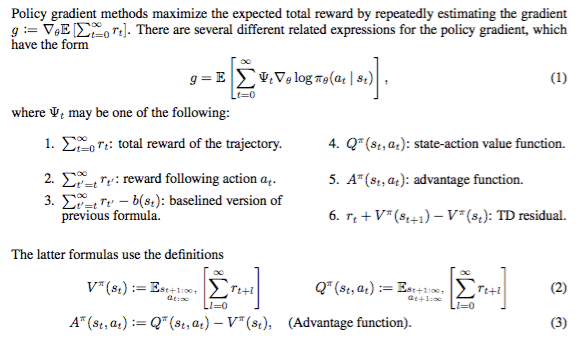Figure 2: Several expressions for the policy gradient from Schulman et al. [4]

Actor-Critic

We can further utilize the value function to improve learning by reducing variance at the cost of introducing bias. Actor-critic methods use the value function to not merely provide a baseline. A “critic” provides a biased value estimate that replaces full sampled returns to guide the policy, which is the “actor”. This approach bootstraps a value estimate using an estimate of the subsequent state value obtained with the same function approximator. Bootstrapping reduces variance to speed up learning, but introduces bias due to reliance on an imperfect critic model.

For example, an actor-critic method can replace the sampled return $R_t$ with an estimate from the temporal-difference (TD) target $r_{t+1} + \gamma V_\omega(s_{t+1})$ using the critic. The network parameters for both the policy (actor) and the value function (critic) are updated with guidance from the critic.

$$\begin{align} &\delta_t = R_t - V_\omega(s_t) \\ &\delta_t = \left[ r_{t+1} + \gamma V_\omega(s_{t+1}) \right] - V_\omega(s_t) \\ &\omega_{t+1} \leftarrow \omega_t + \alpha_\omega \delta_t \nabla_\omega V_\omega(s_t) \\ &\theta_{t+1} \leftarrow \theta_t + \alpha_\theta \delta_t \nabla_\theta \log \pi_\theta(a_t \mid s_t) \end{align}$$

This approach doesn’t require completing a full trajectory like Monte Carlo.

Deep Deterministic Policy Gradients (DDPG)

The actor-critic framework allows us to combine policy gradients with a value-based method like DQN to extend it to continuous action spaces. The techniques introduced in DQN also help deal with issues of error and instability arising from using function approximators with reinforcement learning and policy gradients.

DQN builds on Q-learning (Watkins, 1989), a classic off-policy TD algorithm. Q-learning updates tabular Q-values toward a TD target computed using the action $a = \text{argmax}_{a} Q(s’,a)$ that maximizes the Q-value of the subsequent state.

$$Q(s,a) \leftarrow Q(s,a) + \alpha [r + \gamma \max_a Q(s',a) - Q(s,a)]$$

DQN extended Q-learning using deep neural network function approximators for greater representational capacity to handle high-dimensional state spaces. The DQN paper [2] also introduced experience replay buffers and target networks to stabilize learning.

DDPG (Lillicrap et al., 2016) combines DQN with policy gradient methods using the actor-critic framework to learn a deterministic policy $\mu_\theta(s)$ that acts to approximate Q-learning with guidance from a DQN-like critic $Q_\omega(s,a)$.

Deterministic Policy Gradients (DPG)

Policy gradient methods can model deterministic policies $\mu(s)$ in addition to the stochastic policies $\pi(s \mid a)$ discussed earlier. Deterministic policy gradient methods have better relative sample efficiency since they don’t integrate over action space while stochastic policy methods integrate over both state and action space. The DPG paper (Silver et al., 2014) showed deterministic policy gradients are the expectation of the action value gradient and introduced a deterministic version of the policy gradient theorem to provide an expression for $\nabla_\theta J(\theta)$ that doesn’t require the derivative of the state distribution $\rho^\mu$.

$$\begin{align} &\nabla_\theta J(\mu_\theta) = \mathbb{E}_{s \sim \rho^\mu} \left[ \nabla_{\theta} q^\mu(s,a) \mid _{a=\mu_\theta(s)} \right] \\ &\nabla_\theta J(\mu_\theta) = \mathbb{E}_{s \sim \rho^\mu} \left[ \nabla_\theta \mu_\theta (s) \nabla_a q^\mu (s,a) \mid_{a=\mu_\theta(s)} \right] \end{align}$$

Policy parameters $\theta$ update in proportion to the action value gradient:

$$\theta_{t+1} \leftarrow \theta_t + \alpha_\theta \nabla_\theta \mu_\theta(s) \nabla_a q^\mu(s,a) \mid_{a=\mu_\theta(s)}$$

Deterministic policy gradients work with either on-policy or off-policy approaches. For example, an on-policy SARSA update to the critic takes two determinstic actions per time step, using the second action to estimate the value function in the TD target.

$$\begin{align} &\delta_t = \left[ r_{t+1} + \gamma Q_\omega(s_{t+1},a_{t+1}) \right] - Q_\omega(s_t,a_t) \\ &\omega_{t+1} \leftarrow \omega_t + \alpha_\omega \delta_t \nabla_\omega Q_\omega(s_t,a_t) \end{align}$$

DDPG uses an off-policy approach and computes the TD target using policy $\mu_\theta(s)$, which approximates the maximization in Q-learning.

$$\begin{align} &\delta_t = \left[ r_{t+1} + \gamma Q_\omega(s_{t+1},\mu_\theta (s_{t+1})) \right] - Q_\omega(s_t,a_t) \\ &\omega_{t+1} \leftarrow \omega_t + \alpha_\omega \delta_t \nabla_\omega Q_\omega(s_t,a_t) \end{align}$$

Experience Replay Buffer

DDPG uses experience replay introduced in DQN to collect experience tuples ${(s_i, a_i, s’_i, r_i)}$ in a large memory buffer $\mathcal{B}$. Experiences are sampled for learning update, eliminating temporal correlation of state observations and improving data efficiency by learning from past experiences. Changes in data distribution are also smoothed out by the random sampling from the replay buffer. A common buffer size across literature seems to be 10^6 experience tuples.

Target Networks

DDPG also draws from DQN’s target networks: maintaining a separate copy of the network weights — frozen but periodically updated — for estimating action values in the TD target. The TD target computes an updated value estimate using the latest reward plus a bootstrapped value of the next state. Updating a network based on a target generated from the same evolving network can lead to divergence. Using a frozen or slow changing target network provides a stable fixed target for learning updates by smoothing out short term oscillations.

Soft Updates

Target networks for both actor $\theta’$ and critic $\omega’$ can update using a soft approach, where the target network weights change gradually rather than being frozen and replaced periodically by the current networks $\theta$ and $\omega$.

$$\begin{align} &\theta' \leftarrow \tau \theta + (1-\tau)\theta' \\ &\omega' \leftarrow \tau \omega + (1-\tau)\omega' \end{align}$$

The DDPG paper [6] suggests a hyperparameter value of $\tau=0.001$, while others [8] use $\tau=0.005$.

Batch Normalization

The scale and range of state values can vary significantly due to environmental conditions and differences in units (position, rotation, velocity, angular velocity). Normalizing each dimension to have unit mean and variance across a mini-batch can significantly improve generalization and learning. As suggested in the DDPG paper [6], I apply batch normalization to the state input and before all layers in the actor network. The critic network also uses batch normalization on the state inputs and before all layers not concatenated with action inputs, since we don’t want to alter the action signals.

Exploratory Action Space Noise

Deterministic policies have a harder time attaining sufficient exploration compared to stochastic polices. Continuous action spaces also make exploration important. Adding noise $\mathcal{N}$ directly to the policy helps encourage exploration.

$$\mu'(s_t) = \mu_\theta(s_t) + \mathcal{N}(0,\sigma)$$

The DDPG paper [6] suggests using noise generated from an Ornstein-Uhlenbeck (OU) process so the exploration is temporally correlated. Other researchers [8,11] have found plain Gaussian noise works just as well. After implementating unique OU noise processes for each agent, I’ve also found Gaussian noise with a standard deviation 0.1 works just as well for this robotic arm control task. The actions are clipped between [-1, 1].

Twin Delayed DDPG (TD3)

The TD3 algorithm by Fujimoto et al. in 2018 [8] improves on DDPG with three techniques for handling function approximation error: clipped double Q-learning, delayed policy update, and target policy smoothing.

Clipped Double Q-learning

Q-learning is positively biased due to the max operation used for action selection. For example, taking the max over noisy variables that individually have zero mean can produce an output with positive mean. Double Q-learning (Van Hasselt et al., 2010) and Double DQN (Van Hasselt et al., 2016) deal with the overestimation by maintaining two separate value networks to decouple action selection and evaluation.

Going beyond discrete action spaces, the TD3 paper [8] demonstrates overestimation bias also occurs for continous action spaces in the actor-critic framework. Mitigating bias requires decoupling the action selection (policy) from evalution (value function). We therefore want to use the double Q-learning approach for updating value targets using independent critics.

$$\begin{align} &y_1 = r + \gamma Q_{\omega'_2}(s', \mu_{\theta_1}(s') ) \\ &y_2 = r + \gamma Q_{\omega'_1}(s', \mu_{\theta_2}(s') ) \end{align}$$

However, positive bias still occur for actor-critics with double Q-learning because the critics are not completely independent due to related learning targets and a shared replay buffer. The TD3 paper [8] introduced Clipped Double Q-learning, which uses the minimum of the two critics. The less biased critic becomes upper-bounded by the more biased critic.

$$y_1 = r + \gamma \min_{i=1,2} Q_{\omega'_i}(s', \mu_{\theta_1}(s') )$$

Clipped double Q-learning mitigates overestimation by favoring underestimation. This trade-off makes sense since underestimation bias aren’t prone to spread across learning updates.

Delayed Policy Updates

The TD3 paper [8] highlights the interplay between value and policy updates. Poor value estimates can produce policy updates with divergent behavior. They suggest reducing the frequency of policy updates relative to value updates to allow time for value estimates to improve. This reduces the variance in value estimates used to update the policy, producing a better policy that feeds back into better value estimates. The concept is similar to freezing target networks to reduce error. I use a delay $d=2$ of two critic updates for every actor update as suggested by the TD3 paper [8].

The DDPG paper [6] suggests a soft update hyperparameter $\tau=0.001$ while the TD3 paper [8] uses $\tau=0.005$. Without delayed policy updates, I found $\tau=0.001$ more stable for the Reacher environment. Since the policy update delay also delays the target network updates, I scale $\tau = 0.001d$ in proportion to the delay $d$ to maintain a similar rate of change in the target networks.

Target Policy Smoothing

Deterministic policies can overfit narrow peaks in the value function, increasing variance in the TD target. The TD3 paper [8] address the issue using a regularization technique. Since nearby actions should have similar values, adding some noise to the action in the TD target action evalution should help avoid peaks in the value function.

$$\begin{align} &y = r + \gamma \min_{i=1,2} Q_{\omega'_i}(s', \mu_{\theta'}(s')+\epsilon ) \\ &\epsilon \sim \text{clip}(\mathcal{N}(0,\sigma), -c, c) \end{align}$$

The TD3 paper suggests hyperparamaters of $\sigma=0.2$ clipped at $c=0.5$. For the Reacher environment, I found these settings slowed down learned. Perhaps the noise was too high relative to the action signal range. Scaling down the noise and even using none showed better performance.

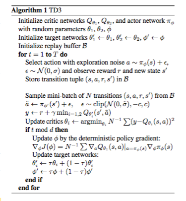Figure 3: TD3 (twin delayed deep deterministic policy gradients) algorithm from Fujimoto et al. [8]

Multi-Step Returns

Monte Carlo methods calculate returns using full trajectories and are unbiased. However, they have high variance and require many samples. One-step TD methods compute a target using the latest reward plus the subsequent state value estimated using a value function approximator. TD methods reduce variance, but the imperfect value function approximator adds bias. Multi-step returns affect the bias-variance trade-off, reducing bias by incorporating reward samples from a longer trajectory into the TD target. The TD target for n-step return generally has the form:

$$y_t = \sum_{i=t}^{t+N-1} \gamma^{i-t} r_{i+1} + \gamma^N V(s_{t+N}, a_{t+N})$$

The TD target for our case with clipped double Q-learning and target policy smoothing becomes:

$$\begin{align} &y_t = \sum_{i=t}^{t+N-1} \gamma^{i-t} r_{i+1} + \gamma^N \min_{i=1,2} Q_{\omega'_i}(s'_{t+N}, \mu_{\theta'}(s'_{t+N})+\epsilon ) \\ &\epsilon \sim \text{clip}(\mathcal{N}(0,\sigma), -c, c) \end{align}$$

Using a 3-step return showed improved learning compared to a standard single step. The D4PG paper by Barth-Maron et al. in 2018 [11] introduced several improvements for DDPG, including using multi-step returns. (The authors also used multiple distributed parallel actors, a distributional critic, and prioritized experience replay.)

Implementation Details

Multiple agents with centralized actor and critic networks

The multiple parallel agents in this version of the Reacher environment collect experiences faster, contributing more samples to the replay buffer and improving exploration. I used centralized actor and critic networks rather than 20 independent actors to reduce computation time.

Network architecture

Architecture for the policy and value networks use suggestions from the DDPG paper [6]. Alternative architectures were not explored here, opting for better generalization rather than fine-tuning for this particular environment. The policy network passes the state input (33 dimensions) into two hidden layers (400 and 300 units) with rectified linear unit (ReLU) activation. State inputs along with inputs to each hidden layer used batch normalization to normalize across mini-batch. Tanh activation on the output produce continous action signals between [-1,1] for each of the four action dimensions.

The value network uses a similar architecture but incorporate action inputs in addition to state inputs to represent $Q_\omega(s,a)$. The state input (33 dimensions) passes to a 400 unit hidden layer with ReLU activation. Four nodes for the action inputs add to the first hidden layer (400 + 4 units) before passing to a second hidden layer (300 units) with ReLU activation. The value network outputs a single unit with ReLU activation to represent $Q_\omega(s,a)$. Only the state inputs and inputs to the first hidden layer with 400 units use batch normalization, which does not make sense for layers downstream of combined state and action inputs.

Clipped double Q-learning involves twin policy and value networks. To reduce computation, the authors [8] suggest using a single policy network. Twin value networks are combined within one network with a single state input head feeding twin value networks, each outputting a separate Q-value. Clipped double Q-learning takes the minimum of the two Q-values to upper-bound the bias with the less biased critic.

Batch size

The policy and value networks learn off-policy by sampling mini-batches from the replay buffer. The DDPG [6] and TD3 [8] papers use batch sizes of 64 and 100, respectively. I found a larger batch size of 256 improves learning, with the drawback of increased computation time. The D4PG paper [11] also used larger batch sizes of 256 and 512.

Network update frequency

To improve learning stability, learning updates occur only every 20 time steps. Each time, the networks update 10 times, each with a new mini-batch sampled from the replay buffer. Using the delayed policy update technique, the actor and both target networks update once for every $d=2$ critic updates to reduced error in the value estimate. The critic network uses only a single gradient step per mini-batch, but perhaps additional gradient steps would produce a worthwhile improvement to the value estimate.

Gradient clipping

Gradient clipping for the critic helps stabilize learning by prevent gradients from becoming too large.

Initial random exploration

Agents take random actions for the initial 5000 time steps to improve exploration and reduce dependency on initial network weights.

Adam optimizer weight decay

The DDPG paper [6] suggested using Adam optimization with zero weight decay for the actor and 0.01 for the critic. A critic weight decay of 0.0001 worked much better for this case.

Training the Agent

Let’s train an agent for the Reacher environment. Success requires a score of 30 (average across all 20 agents) over 100 episodes.

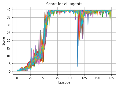
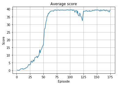
The learning curve shows the agent surpasses an average score of 30 around episode 55 and maintains a higher average thereafter, successfully accomplishing the continous control task. We see a dip in learning between epsiodes 110 and 125, but the average score stays above 30 and the agent recovers.

As a sanity check, let’s examine the action values and rewards by sampling from the replay memory.

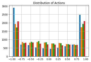
The action histogram shows a reasonable distribution of actions across the continuous range between [-1,1]. Most actions occur at the min and max limits, but a good portion occur in between. This also suggests the action space noise is scaled sensibly.

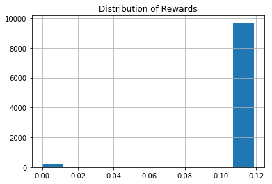
The reward histogram shows the vast majority of transitions result in positive rewards. A very small number have zero reward. Positive rewards begin at 0.04 points. The histogram actually shows the multi-step discounted return used in the TD target, so we mostly see a return of 0.12 points in accordance with a 3 step trajectory.

Testing the Agent

Now let’s use the trained agent to interact with the Reacher environment.

The GIF animation in Figure 1 previews the first several time steps, but here’s a full video showing the trained agent across 1000 time steps: https://youtu.be/JC9iwMmjpzo.

Discussion & Next Steps

We successfully built an agent trained using a multi-step variant of twin delayed DDPG to track a moving target using a robotic arm. We see the agent learns to quickly move the arm into the target region and track the moving target regardless of how fast or slow it moves.

Learning instabilities added a fair amount of challenge. Adjusting the network update frequency helped stabilize learning. Efforts to ensure good value estimation from the critic — reducing overstimation bias, using more critic updates, and adjusting the critic weight decay — were helpful in improving learning.

The next steps involve comparing learning performance across multiple random seeds and checking how the current approach generalizes to other environments beyond Reacher. For example, target policy smoothing did not seem to improve learning in Reacher. Would it help in another environment?

Also, many techniques were applied in combination to this learning task. Performing an ablation study would provide valuable insight into the impact of individual techniques. For example, how much did using a multi-step return method help? How important was using clipped double Q-learning? The present work was performed on a laptop, so running these ablation studies across multiple random seeds would require more time and computational resources.

The current work uses action space noise for exploration. Researchers [12] have demonstrated good results with parameter space noise, another promising technique worth implementing.

Explore the code and reproduce these results for yourself here: supercurious/deep-rl-continuous-control

References

1. https://github.com/Unity-Technologies/ml-agents

2. Mnih, Volodymyr, Kavukcuoglu, Koray, Silver, David, Rusu, Andrei A., Veness, Joel, Bellemare, Marc G., Graves, Alex, Riedmiller, Martin, Fidjeland, Andreas K., Ostrovski, Georg, Petersen, Stig, Beattie, Charles, Sadik, Amir, Antonoglou, Ioannis, King, Helen, Kumaran, Dharshan, Wierstra, Daan, Legg, Shane, and Hassabis, Demis. Human-level control through deep reinforcement learning. Nature, 518(7540):529–533, 02 2015. URL http://dx.doi.org/10.1038/nature14236.

3. Sutton, R. and Barto, A. Reinforcement Learning: An Introduction. MIT Press. 1998.

4. Schulman, John, Moritz, Philipp, Levine, Sergey, Jordan, Michael, and Abbeel, Pieter. High-dimensional continuous control using generalized advantage estimation. arXiv preprint arXiv:1506.02438, 2015b.

5. Watkins, C.J.C.H. (1989), Learning from Delayed Rewards (Ph.D. thesis), Cambridge University, 1989. URL http://www.cs.rhul.ac.uk/~chrisw/new_thesis.pdf

6. Lillicrap, T. P., Hunt, J. J., Pritzel, A., Heess, N., Erez, T., Tassa, Y., Silver, D., and Wierstra, D. Continuous control with deep reinforcement learning. arXiv preprint arXiv:1509.02971, 2015.

7. Silver, D., Lever, G., Heess, N., Degris, T., Wierstra, D., and Riedmiller, M. Deterministic policy gradient algo- rithms. In International Conference on Machine Learning (ICML), 2014.

8. Fujimoto, S., van Hoof, H., and Meger, D. Addressing function approximation error in actor-critic methods. arXiv preprint arXiv:1802.09477, 2018.

9. Hasselt, H. V. Double Q-learning. In Advances in Neural Information Processing Systems (NIPS), pp. 2613–2621, 2010.

10. Van Hasselt, Hado, Guez, Arthur, and Silver, David. Deep Reinforcement Learning with Double Q-learning. In Proceedings of the Thirtieth AAAI Conference on Artificial Intelligence, 2016. URL http://arxiv.org/abs/1509.06461.

11. Barth-Maron, G., Hoffman, M. W., Budden, D., Dabney, W., Horgan, D., TB, D., Muldal, A., Heess, N., and Lillicrap, T. Distributional policy gradients. In Proceedings of the International Conference on Learning Representations (ICLR), 2018.

12. https://blog.openai.com/better-exploration-with-parameter-noise/