Building Intuition for Softmax, Log-Likelihood, and Cross Entropy

Softmax, log-likelihood, and cross entropy loss can initially seem like magical concepts that enable a neural net to learn classification. Modern deep learning libraries reduce them down to only a few lines of code. While that simplicity is wonderful, it can obscure the mechanics. Time to look under the hood and see how they work! We’ll develop a deeper intuition for how these concepts enable neural nets to perform challenging tasks like recognizing dog breeds or even expert-level diagnosis on whether a skin lesion could be cancerous. Starting from raw network outputs, we’ll explore and visualize how softmax, negative log-likelihood, and cross entropy loss can turn an untrained neural net into a well-trained classifier.

Let’s consider training a neural net to identify numbers by showing it images of handwritten digits from the MNIST dataset. Using a simple architecture, we can accomplish the task with high accuracy without anything fancy. We feed every pixel value of an image into a single hidden layer with ReLU activation. ReLU merely converts any negative values to zero. The hidden layer feeds into an output layer consisting of ten outputs, since we want to classify our images as one of ten numbers from 0 to 9.

Tutorials from Tensorflow and PyTorch commonly use MNIST to demonstrate image classification. The Tensorflow tutorial code in Figure 1 defines a softmax activation on the final layer, along with a cross entropy loss function. In PyTorch, you can simply define a cross entropy loss function that takes in the raw outputs of your network and compares them with the true labels. Let’s look closely at what exactly flows out of the network to make these predictions and how that changes during training.

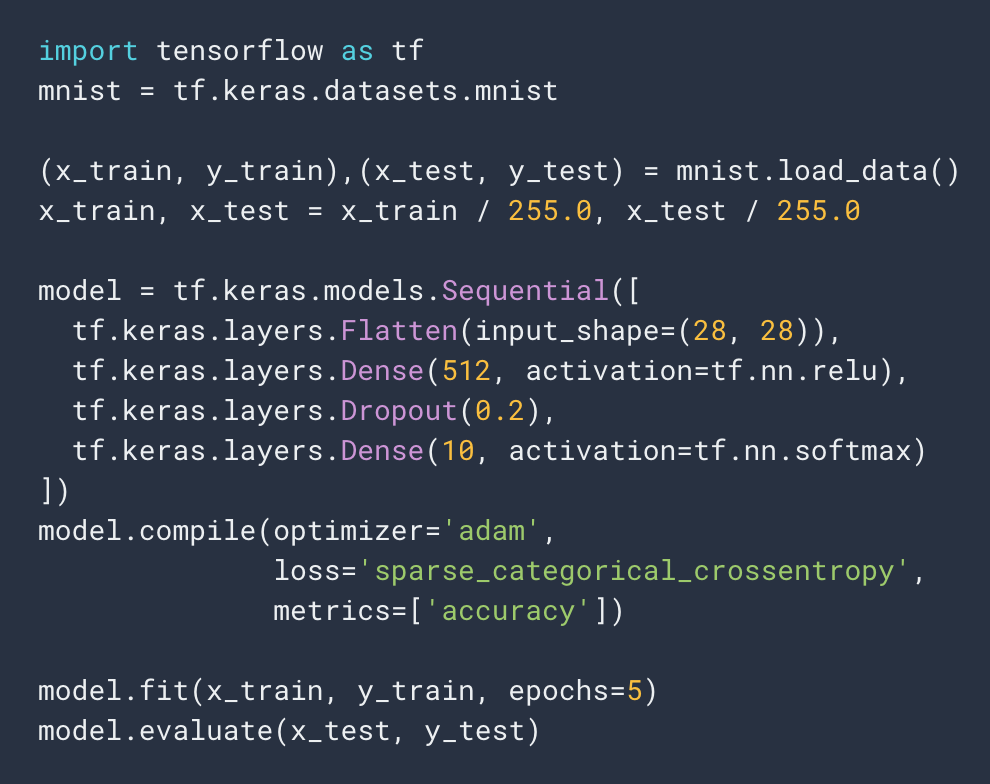Tensorflow code Figure 1: Tensorflow tutorial code for training an image classifier on the MNIST dataset.

Visualizing raw outputs from the network

What do the raw outputs from the neural net look like? How do the outputs respond to different input classes? We can visually answer this question by feeding in image samples of the same digit class and using histograms to plot the raw outputs (sometimes called logits). Figure 2 shows the output distributions when the network sees image samples for a particular handwritten digit. The ten colors correspond to the ten network outputs. We haven’t trained the network yet, so the outputs look about the same whether we give it 0’s or 1’s or any other input class. These outputs are currently just a function of the randomly initialized network parameters.

How would this look like for a trained network? Figure 3 shows the output from a trained network. We can see more structure now. Most of the output distributions are still clumped together, but one particular distribution clearly stands out with the highest value: the distribution corresponding to the input class. The network has learned to produce higher values for the output matching the input class.

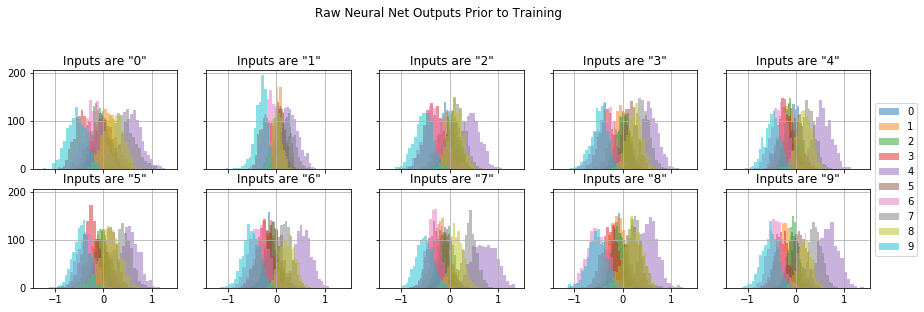Raw output distribution (untrained) Figure 2: Each plot shows the raw network output distribution for all ten outputs when fed image samples of the same handwritten number. Each color corresponds to one of network’s ten outputs. We haven’t trained the network yet, so the outputs are random.

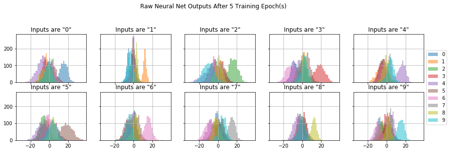Raw output distribution (trained) Figure 3: Each plot shows the raw network output distribution for all ten outputs when fed image samples of the same handwritten number. Each color corresponds to one of network’s ten outputs. The network has gone through some training. The distribution with the highest value (along the x-axis) corresponds to the true class of the input image.

So how do we formulate a loss function to train the network to go from Figure 2 (untrained randomness) to Figure 3 (trained to output the highest value for the input class)? It’s not enough to merely know whether the prediction is correct or not; we need the loss function to tell us how far the prediction is from the truth. Knowing how far off our prediction is, we can iteratively update our network parameters to minimize error and make better predictions across optimization steps.

Softmax

Now let’s bring in softmax. The softmax function maps raw network outputs to a probability distribution. In other words, softmax transforms each of the ten outputs to a value between 0.0 and 1.0, with all ten summing to 1.0. After training, the probability will be higher for the predicted class and lower for the others.

Let’s now visualize the output distributions using box plots rather than histograms to better see and compare the median value across outputs. Figure 4 shows the distribution for each output class when fed image samples of the same class: handwritten 1’s. Softmax takes in the raw outputs from the left plot and produces the probabilities in the right plot. The top two plots show an untrained network. The softmax medians (orange lines) hover around 0.1 because the untrained network predicts roughly an equal probability of 1/10 across our ten classes. In contrast, the trained network in the bottom plots has learned to assign a high probability near 1.0 to class 1 (since we’re feeding in handwritten 1’s) and low probabilities near 0.0 to the other classes.

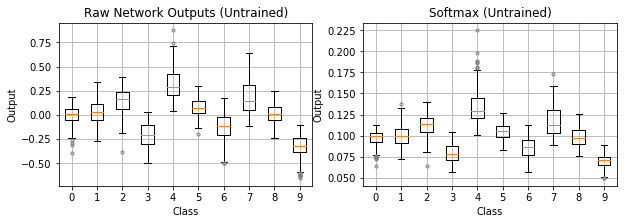
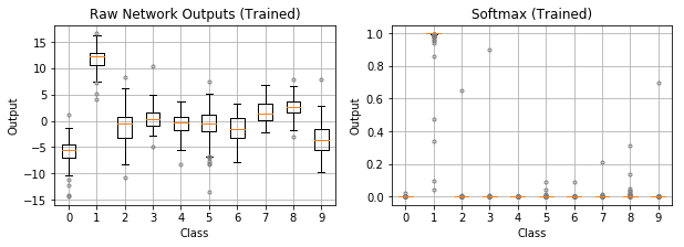Logits to Softmax (Untrained) Logits to Softmax (Trained) Figure 4: The softmax function maps raw network outputs to a probability distribution. The top plots show an untrained network and the bottom plots show a trained network. Samples of handwritten 1’s are fed to the network. When untrained, the probabilities produced from softmax hover around 1/10. When trained, softmax produces a probability near 1.0 for class 1 and low probabilities near 0.0 for other classes.

Mathematically, softmax is defined as follows. For raw network outputs across $C$ classes $\mathbf{x} = (x_1, …, x_C) \in \mathbb{R}^C$ and class $i = 1, …, C$,

$\text{softmax}(\mathbf{x})_i = \frac{e^{x_i}}{\sum_{j=1}^C e^{x_j}}$

In other words, softmax takes the exponential of the each raw output and normalizes by the sum of the exponentials across class. The exponential function (Figure 5) increases monotonically and is positive, which is important because the raw network outputs can be negative. The exponential function also boosts the highest output by making it exponentially higher than the rest. Lastly, normalizing by the sum of exponentials across class ensures all softmax outputs sum to 1.0, forming a probability distribution.

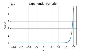Figure 5: The exponential function is monotonic, outputs positive values, and boosts the highest value.

Log of probabilities

Taking the log of probabilities makes them easier to work with for many reasons:

Logarithms convert very small probabilities into larger (negative) numbers. The log plot in Figure 6 shows tiny probabilities near 0.0 map to larger and more numerically manageable negative values. Computers have finite precision, so working with the log reduces underflow and improves numerical stability. You can always convert back to probability by using the exponential function.
Logarithms are monotonically increasing functions, so optimizing the log of a function is the same as optimizing the function itself.
Logarithms offer mathematical convenience, such as turning multiplication into addition and division into subtraction.

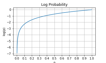log(x) Figure 6: Log of probabilities between 0.0 and 1.0. Probability values can become very small, especially when a trained neural net is confident in the low probability of a class. Taking the log converts that tiny number into a larger, more numerically manageable number.

For these benefits, we take the log of the softmax function. In fact, Tensorflow has a specific function for log softmax (tf.nn.log_softmax) and so does PyTorch (torch.nn.LogSoftmax).

Log-likelihood loss

Log probability also has a useful property: starting on the right of Figure 6 from a probability of 1.0 and decreasing left toward a probability of 0.0, the log goes from $\log(1.0) = 0$ and changes exponentially in magnitude. The behavior is quite suitable for expressing the loss of a predicted probability for a class. For example, a predicted probability near 1.0 for the true class – a confident and accurate prediction – would produce a loss near zero. As the predicted probability for that true class drops toward zero, the loss magnitude increases exponentially. Such a loss function discourages wrong predictions, especially confident wrong prediction. This loss function is called log-likelihood loss.

Let’s visualize the progression from raw outputs to softmax to log softmax (Figure 7). Because the untrained network gives each classes roughly an equal 1/10 probability, the log softmax values hover around $\log(0.1) = -2.3$. The training process would then attempt to bring this loss of about -2.3 toward zero.

The trained network in the bottom plots has learned the images are handwritten 1’s. Class 1 has a high softmax probability near 1.0, translating to a log softmax near 0.0. That’s a good loss value for the correct prediction. The rest of the softmax probability distribution goes to the other classes, which have very small probabilties near zero. Log softmax converts them to numerically friendly larger magnitude values around -15 to -20. These would be huge loss values relative to the initial loss of -2.3. However, since these other classes have zero probability of being the true class, their losses shouldn’t have any weight.

So how exactly do we combine the log probabilities across classes into a single loss value? The log probabilities should only contribute to the loss in proportion to the true probability of their respective class. In other words, our measure of loss (log probability) should be weighted by the probability distribution of the ground truth. For our image classification example, the math simplifies since only one of the classes has a true probability of 1.0 while others are all zero. Therefore, only the log probability for the single true class should count toward loss.

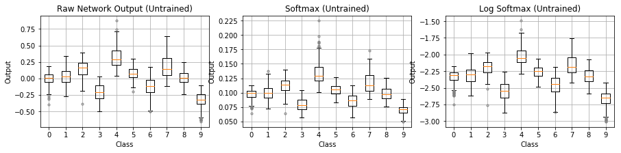
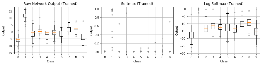Log Softmax (untrained) Log Softmax (trained) Figure 7: Going from raw outputs, to softmax, to log softmax.

A final tweak on log softmax is taking the negative of the log probabilities. This is also called the negative log-likelihood loss or log loss. In PyTorch, it is torch.nn.NLLLoss. Remember, our loss values are currently negative because log produces negative values between 0.0 and 1.0 (Figure 6). We’ve been talking about increasing the loss from initially -2.3 up to zero. Most optimizers, however, work by minimizing a loss function rather than maximizing. By taking the negative of log probabilties, the optimizer can work to minimize the initial loss of $-\log(0.1) = 2.3$ (the red dot in Figure 8) down to zero (green dot) as it learns to predict the correct class with high confidence. To illustrate this in practice, Figure 9 shows losses across a batch of images before training and after. The average loss over the batch starts at ~2.3 and drops near zero after training.

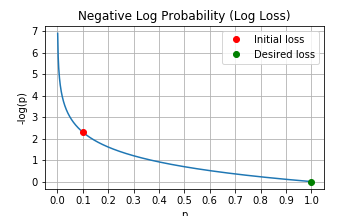Figure 8: Negative log probability as a loss function. A untrained network predicts roughly equal probability of 1/10 across the 10 classes. The loss starts at -log(0.1) = 2.3 (red dot) and minimizes during training toward -log(1.0) = 0 (green dot).

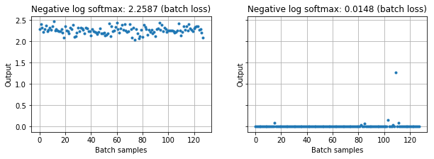Loss before and after training Figure 9: Loss over a batch of images before and after training. Losses begin at values near -log(0.1) = 2.3 and drop toward zero after training.

Cross entropy loss

So what about cross entropy loss? Cross entropy is a concept from the field of Information Theory. For a great explanation, I recommend Chris Olah’s Visual Information Theory where he says “cross entropy gives us a way to express how different two probability distributions are.” When applied to machine learning as a loss function, cross entropy loss can compare a predicted probability distribution to a true probability distribution. You multiply the true probabilities by the log of the predicted probabilities, sum across class, and take the negative. Mathematically, cross entropy loss is expressed as follows. For true probabilities $y_i$, predicted probabilities $p_i$, and class $i$ out of $C$ total classes, cross entropy loss $L_{ce}$ is:

$L_{ce} = -\sum_{i=1}^C {y_i \log p_i}$

It’s essentially the negative sum of the log of predicted probabilities, weighted by the true probability. Sound familiar? We just did it! We used softmax to get predicted probabilities. We used the negative log-likelihood loss function by taking the negative log of probabilities to express a loss value to minimize. We then reasoned that the individual log loss values across our ten output classes should only contribute to the loss in proportion to their true probability distribution. This comparison between two probability distributions is what cross entropy loss measures. In our example, a single class has a true probability of 1.0, which simplifies the math quite a bit. However, you can begin to see how this concept is useful for comparing two probability distributions.

Closing thoughts

We started with a basic network architecture with a single hidden layer. We investigated the raw outputs from the network and casted them as a probability distribution using the softmax function. We leveraged the properties of logarithms to formulate a measure of loss (log-probability) that would be near zero for a correct and confident prediction while growing exponentially with increasing error. We took the negative of log probability to express a loss function suitable for minimization by the optimizer. We reasoned that log probabilities for each class should only contribute to the loss in proportion to the true probability of that class, arriving at cross entropy loss. We also demonstrated how optimizing network parameters to decrease this loss produced a well-trained image classifier.

This approach of visualizing raw network outputs, examining function characteristics, and reasoning about loss contributions was useful to me for building intuition about softmax, log-likelihood, and cross entropy loss. I hope you found it valuable as well. If I’m missing anything here or you’ve come across insightful explanations on this topic, please let me know!

Explore the code and reproduce these results for yourself in this notebook: supercurious/softmax-cross-entropy